Evolution involves a random process. Richard Harris compares the mathematics to that of blind chance.
On the 28th May 2007, the Creation Museum [ Creation ] opened its doors to the public for the first time. Located in Kentucky USA, its purpose is to present scientific evidence in support of the thesis of Young Earth Creationism. This holds that Genesis is a literal account of the creation of the universe, that the Earth was created in six days between six and ten thousand years ago, that fossil beds were laid down during the flood and that human evolution is unsubstantiated religious doctrine. They propose that an international conspiracy of politically motivated secular humanists have duped the people of the world into accepting their faith as scientific truth [ MatriscianaOakland91 ].
I must say that I find the claims of an international conspiracy somewhat surprising; I've certainly never been invited to contribute. That said, being a secular humanist unmotivated to the verge of apathy, I'd probably be the last person they'd want to enlist.
I can understand the doubt many creationists have that evolution can account for the rich array of complex life we find surrounding us. After all, it's fundamentally a random process and life exhibits a remarkable degree of organisation.
William Paley [ Paley02 ] famously expressed this doubt by pointing out that if we were to come across a watch lying upon the ground, we should inevitably deduce the existence of a watchmaker. Richard Dawkins rejoinders this in his book The Blind Watchmaker [ Dawkins86 ] with the familiar argument that it is the accumulation of small beneficial random changes rather than single large random changes that account for the emergence of order.
Unsurprisingly, my first instinct is to construct a simple model to investigate this argument.
I propose that we model iterated improvement by measuring how long it takes to randomly count from zero to a given threshold, t , in the range [0, n). I use the term randomly counting to describe subtracting one, doing nothing or adding one with equal probability and choosing the better of the original and the changed value 90% of the time. In other words we have six possible outcomes, as illustrated in Figure 1.
|
|
|||||||||||||||||||||||||||
| Figure 1 |
For comparison we will randomly select numbers from the range and measure how long it takes before we have one greater than or equal to the threshold.
There will be no need to run any simulations since the model is so simple that a comprehensive probabilistic analysis is relatively straightforward.
Let's start with the second of these; the number of times we need to randomly select numbers before we reach the threshold.
There are n - t numbers greater than or equal to t in the range. The probability of picking one of these is therefore
![]()
The expected number of steps before we reach the threshold is simply the reciprocal of this probability.
![]()
To calculate the number of steps that iterated improvement requires, we should note that the expected increase from each step can be found by multiplying the value of each step by the probability that we take it and summing them. For simplicity, we'll allow the value to step below zero, so that every step is the same.
The expected number of steps is then the threshold divided by the expected step increase.
This doesn't look good for iterated improvement. It will only take fewer steps than the totally random scheme if
![]()
Rearranging, we find that we require
Now, since t is strictly less than n , the right hand is smaller than the left for most choices of n and t , and hence iterated improvement is generally going to be even worse than random sampling. To make this absolutely clear let's pick some specific values, say one hundred for n and fifty for t .
I think that this demonstrates the point; iterated improvement is not enough to explain why evolution should be any more effective than guesswork.
So does this weaken the argument for evolution?
Well, no. It does highlight a significant weakness in my model however.
A better model would reflect the fact that evolution operates upon many different attributes simultaneously. We can extend our model to account for this by using a d dimensional vector of integers instead of a single integer.
This time each step will randomly change the value of every element and we will consider the result to be a retrograde step if any of the elements are smaller than they were.
Given that the each element is changed independently of the others, the expected number of random guesses we need to take before every element is greater than the threshold is simply the product of the expected number of guesses needed for each of them.
![]()
With iterated improvement the calculation is slightly more complicated. We can still exploit the independence of the elements since every element will have the same expected increase at each step.
If the given element takes a positive step, it will be considered a success only if all of the remaining elements do not take a negative step. Once again we can exploit the independence of the elements by simply multiplying the probabilities that each of them is not negative.
![]()
The probability of any of the remaining elements taking a retrograde step is simply one minus this.
![]()
The probability that an element takes a positive step is therefore
If an element takes a negative step, the whole step is necessarily considered retrograde. The probability of taking it is therefore
![]()
The expected increase of an element from each step is therefore
Since all of the elements change at the same rate, the expected number of steps needed for every element to reach the threshold is simply the threshold divided by d.
![]()
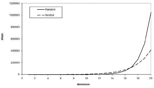
So the advantage of iterated improvement is that, for a sufficiently large threshold, it scales far better than random guessing does as the number of dimensions increases. Note that sufficiently large means greater than just one third of the upper bound. Using the same values for t and n as before, Figure 2 illustrates the expected number of steps each scheme requires various numbers of dimensions.
|
| Figure 2 |
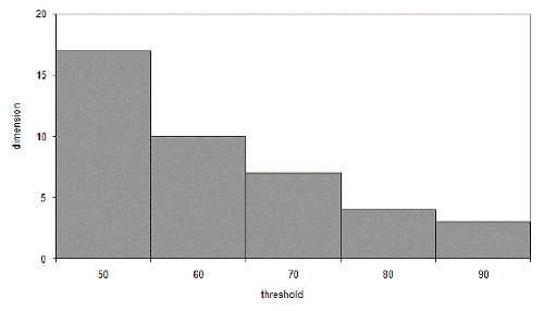
At seventeen dimensions, iterated improvement becomes more efficient than simple random sampling. This may seem like a lot, but the threshold we chose wasn't particularly high. Figure 3 illustrates the dimensions at which iterated improvement is better than sampling for various thresholds for our n of one hundred.
|
| Figure 3 |
One criticism of this as a model for evolution is that the rate of change is rather rapid and that the better candidate is selected far more often than would be expected in reality. However, if we consider each step to be the cumulative result of many generations, these choices start to look more reasonable.
We can illustrate this by performing the same analysis using different probabilities of change and selection, say 1% chance of improvement, 1% chance of degradation and 51% chance of selecting the better of the two vectors. This yields an expected increase per step of
![]()
The proportional change in the number of steps we need to take before we have the same expected increase as before is simply the original expected increase divided by this new one
Whilst this may seem like a large number, it reduces rather quickly as the number of dimensions increases. Furthermore, even the worst factor of approximately 1,667 would result in one aggregate step in as little as 40 weeks for bacteria with a reproduction rate of one generation per hour.
The stated position of Answers in Genesis [ Genesis ], the owners of the Creation Museum, is that evolution is true, but in a limited form. They make the distinction between evolution within a species, called microevolution, and the evolution from one species to another, called macroevolution. They accept that the former is true, it can be observed in the adaptation of bacteria to antibiotics for example, but reject the latter claiming that nobody has ever seen one species evolve into another.
One of the arguments they use to refute the suggestion that given sufficient time a large number of small changes will accumulate into a large change is the assertion that evolution can only remove information, not create it.
In this light, it could be argued that my model presupposes the goal, that the answer I seek is encoded into the very vector that is subjected to iterated improvement; counting is, after all, what integers are for .
To investigate this, we'll need some code with which to run experiments.
To begin with we'll need a source of random numbers. The one we used in our last project will be fine and is reproduced in Listing 1.
    double
    rnd(double x)
    {
      return x * double(rand())/
         (double(RAND_MAX)+1.0);
    }
|
| Listing 1 |
Next, we'll need a class to represent one of our hypothetical creatures. In a fit of originality, I've called it individual and its definition is given in Listing 2.
    namespace evolve
    {
      class individual
      {
      public:
        typedef biochem::genome_type  genome_type;
        typedef biochem::phenome_type phenome_type;
        individual();
        explicit individual(const biochem &b);
        const individual & operator=(
           const individual &other);
        void               reset();
        const genome_type &  genome() const;
        const phenome_type & phenome() const;
        void swap(individual &other);
        void reproduce(individual &offspring) const;
      private:
        void develop();
        void mutate();
        const biochem * biochem_;
        genome_type     genome_;
          phenome_type    phenome_;
      };
    }
|
| Listing 2 |
The thus far undefined biochem class is an interface class that we will use to abstract the details of the model, allowing us to fiddle with them without rewriting all of our code. Before discussing the individual class further it's probably worth taking a look at the definition of the biochem class, given in Listing 3.
    namespace evolve
    {
      class biochem
      {
      public:
        typedef
           std::vector<unsigned long> genome_type;
        typedef
           std::vector<double>        phenome_type;
        virtual size_t genome_base() const = 0;
        virtual size_t genome_size() const = 0;
        virtual size_t phenome_size() const = 0;
        virtual double p_select() const = 0;
        virtual void develop(
           const genome_type &genome,
           phenome_type &phenome) const = 0;
      };
    }
|
| Listing 3 |
We represent the genetic makeup of our model individuals with the genome_type defined here and their features with the phenome_type . These terms, like many I shall use in this project, originate from the field of biology. The important thing to note about them is that the genetic makeup is discrete in nature (i.e. integer valued) whereas the features are continuous (i.e. floating point valued).
The genome_size and phenome_size member functions determine the size of the two vectors. The genome_base member function determines the range of integers that constitute the elements of the genome. The develop member function maps a particular genetic makeup to a set of features. Finally, the p_select member function indicates the probability that we select the better of two individuals; remember that this was 0.9 in our original analysis.
In addition to managing the representation of the genome and phenome, the individual class is responsible for the reproductive process. As in our earlier analysis this involves a random change to a single element of the genetic makeup.
Before we can do this, however, we must initialise the individual so let's begin by taking a look at the constructors (Listing 4).
    evolve::individual::individual() : biochem_(0)
    {
    }
    evolve::individual::individual(
       const biochem &biochem) : biochem_(&biochem),
       genome_(biochem.genome_size(), 0)
    {
      develop();
    }
|
| Listing 4 |
An interesting point to note is that whilst we pass the biochem by reference we store it by pointer. This is because we will want to store individual s in standard containers and they require contained classes to be both default initialisable and assignable. These are tricky properties to support for classes with member references since, unlike pointers, they cannot be re-bound.
Note that by default, we initialise the genome with 0 . If we want to randomly initialise the individual , we need to call the reset member function, illustrated in Listing 5.
    void
    evolve::individual::reset()
    {
      if(biochem_->genome_base()<2)
         throw std::logic_error("");
      genome_type::iterator first = genome_.begin();
      genome_type::iterator last  = genome_.end();
      while(first!=last)
      {
        *first++ = (unsigned long)rnd(double(
           biochem_->genome_base()));
      }
      develop();
    }
|
| Listing 5 |
The reset function is pretty straightforward; it simply sets each element of the genome to a random number picked from zero up to, but not including, genome_base .
Like the constructor, it ends with a call to the develop member function. This is responsible for mapping the genome to the phenome and is shown in Listing 6.
    void
    evolve::individual::develop()
    {
      if(biochem_==0) throw std::logic_error("");
      biochem_->develop(genome_, phenome_);
    }
|
| Listing 6 |
This simply forwards to the biochemistry object which will initialise the phenome according to whatever plan we wish.
Now we're ready to take a look at the reproduce member function. As Listing 7 illustrates, this simply copies the individual to an offspring and subsequently mutate s and develop s it.
    void
    evolve::individual::reproduce(
       individual &offspring) const
    {
      if(biochem_==0) throw std::logic_error("");
      offspring.biochem_ = biochem_;
      offspring.genome_.resize(genome_.size());
      std::copy(genome_.begin(), genome_.end(),
                offspring.genome_.begin());
      offspring.mutate();
      offspring.develop();
    }
|
| Listing 7 |
Note that we use resize and copy rather than assignment since for most of our simulation the offspring will already be the correct size, so we may as well reuse its genome_ .
So the final member function of interest is therefore mutate . This simply picks a random element of the genome and, as in our earlier analysis, with equal probability increments, decrements or leaves it as it is (Listing 8).
    void
    evolve::individual::mutate()
    {
      if(biochem_==0) throw std::logic_error("");
      if(biochem_->genome_base()<2)
         throw std::logic_error("");
      size_t element =
         size_t(rnd(double(genome_.size())));
      size_t change  =
         biochem_->genome_base()+size_t(rnd(3.0))-1;
      genome_[element] += change;
      genome_[element] %= biochem_->genome_base();
    }
|
| Listing 8 |
We decide on the change we'll make to the selected element by generating a random unsigned integer less than three and subtracting one from it, leaving us with either minus one, zero or plus one. To ensure that we don't underflow the element if we try to decrement below zero, we add genome_base to the change, d . Since the change is ultimately made modulo genome_base to ensure that the changed element remains in the valid range this is cancelled out at the end of the calculation.
So now that we have a class to represent individual creatures we need a class to maintain a collection of them which, in another display of stunning originality, I will call population (Listing 9).
    namespace evolve
    {
      class population
      {
      public:
        typedef std::vector<individual>
           population_type;
        typedef population_type::const_iterator
           const_iterator;
        population(size_t n, const biochem &b);
        size_t             size() const;
        const individual & at(size_t i) const;
        const_iterator     begin() const;
        const_iterator     end() const;
        void reset();
        void generation();
      private:
        void               reproduce();
        void               select();
        const individual & select(const individual &x,
           const individual &y) const;
        const biochem & biochem_;
        population_type population_;
        population_type offspring_;
      };
    }
|
| Listing 9 |
Whilst the basic purpose of the population class is to maintain a set of individual s, it is also responsible for managing the steps of the simulation. It does this with the generation member function which controls the reproduction and selection of individual s.
We initialise the population class with the constructor (Listing 10).
    evolve::population::population(size_t n,
       const biochem &biochem) :biochem_(biochem),
       population_(n, individual(biochem_)),
       offspring_(2*n)
    {
      reset();
    }
|
| Listing 10 |
Note that, unlike for individual , we store the biochem by reference. This is because we will not need to store population objects in standard containers.
The constructor initialises the population_ member with n biochem_ initialised individual s and the offspring_ member with 2*n uninitialised individual s. The former represents the population upon which we will perform our simulation, whilst the latter provides a buffer for the reproduction and selection process.
Finally, the constructor calls the reset member function to randomly initialise the population (Listing 11).
    void
    evolve::population::reset()
    {
      if(biochem_.genome_base()<2)
         throw std::logic_error("");
      population_type::iterator first =
         population_.begin();
      population_type::iterator last  =
         population_.end();
      while(first!=last) first++->reset();
    }
|
| Listing 11 |
The reset member function simply iterates over population_ calling reset to randomly initialise each member.
As mentioned above the final member function, generation , is responsible for running each step of the simulation and it is illustrated in Listing 12.
    void
    evolve::population::generation()
    {
      reproduce();
      select();
    }
|
| Listing 12 |
This simply forwards to the reproduce and select member functions. The former is responsible for reproducing each individual in the population_ member into two individual s in the offspring_ buffer. The latter is responsible for competitively selecting members of the offspring_ buffer back into the population_ (Listing 13)
    void
    evolve::population::reproduce()
    {
assert(2*population_.size()==offspring_.size());
      population_type::const_iterator first =
         population_.begin();
      population_type::const_iterator last  =
         population_.end();
      population_type::iterator out =
         offspring_.begin();
      while(first!=last)
      {
        first->reproduce(*out++);
        first++->reproduce(*out++);
      }
    }
|
| Listing 13 |
Again, this is a relative simple function since the reproduction of each individual is delegated to the individual itself.
The select member function is a little more complex (Listing 14).
    void
    evolve::population::select()
    {
assert(offspring_.size()==2*population_.size());
      population_type::iterator first =
         offspring_.begin();
      population_type::iterator last  =
         offspring_.end();
      population_type::iterator out   =
         population_.begin();
      std::random_shuffle(first, last);
      while(first!=last)
      {
        const individual &x = *first++;
        const individual &y = *first++;
        if(x.genome().size()!=y.genome().size())
        {
          throw std::logic_error("");
        }
        if(x.phenome().size()!=y.phenome().size())
        {
          throw std::logic_error("");
        }
        *out++ = select(x, y);
      }
    }
|
| Listing 14 |
The select member function ensures that every offspring competes for inclusion in the new population. It does this by randomly reordering them, using std::random_shuffle , and then having each adjacent pair compete for selection (Listing 15).
    const evolve::individual &
    evolve::population::select(const individual &x,
       const individual &y) const
    {
      if(x.phenome().size()!=y.phenome().size())
      {
        throw std::logic_error("");
      }
      double px = 0.5;
      if(pareto_compare(y.phenome().begin(),
         y.phenome().end(), x.phenome().begin(),
         x.phenome().end()))
      {
        px = biochem_.p_select();
      }
      else if(pareto _compare(x.phenome().begin(),
         x.phenome().end(), y.phenome().begin(),
         y.phenome().end()))
      {
        px = 1.0 - biochem_.p_select();
      }
      return (rnd(1.0)<px) ? x : y;
    }
|
| Listing 15 |
This competitive selection more or less follows the scheme we used in our initial analysis. The main difference is rather than having an offspring compete with its parent, we now have offspring competing against each other.
To this end, we simply select the better of the two individual s, as determined by the pareto_compare function, with the probability given by the biochem_ . The pareto_compare function returns true if each element in the first iterator range is strictly less than the equivalent element in the second range.
The terminology originates in mathematics. If we take a set of points in more than one dimension, those that are not less than any of the others in the set on at least one axis are known as the Pareto optimal front and represent the set of valid trade offs between the values on each axis. For example, if we had two values representing the efficiency and power of an engine, we may be willing to sacrifice power for the sake of efficiency, or efficiency for the sake of power. All other things being equal, we should not compromise on both. The Pareto optimal front therefore gives us the set of acceptable compromises.
Figure 4 illustrates the Pareto optimal front for a set of points randomly distributed inside a quarter circle.
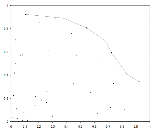
|
| Figure 4 |
The signature of the pareto_compare function is inspired by std::lexicographical_compare and since it must therefore deal with ranges of different lengths is a little more general than we require. We deal with ranges of different lengths by hypothetically extending the shorter range with values strictly less than those in the longer range. In practice this means if we reach the end of the first range without encountering an element not less than one from the second range, the first range is considered lesser than, or in mathematical parlance dominated by, the second (Listing 16).
    namespace evolve
    {
      template<class InIt1, class InIt2>
        bool pareto_compare(InIt1 first1, InIt1 last1,
           InIt2 first2, InIt2 last2);
    }
    template<class InIt1, class InIt2>
    bool
    evolve::pareto_compare(InIt1 first1, InIt1 last1,
       InIt2 first2, InIt2 last2)
    {
      while(first1!=last1 && first2!=last2 &&
         *first1<*first2)
      {
        ++first1;
        ++first2;
      }
      return first1==last1;
    }
|
| Listing 16 |
    namespace evolve
    {
      template<class InIt1, class InIt2, class Pred>
         bool pareto_compare(InIt1 first1, InIt1 last1,
         InIt2 first2, InIt2 last2, Pred pred);
    }
    template<class InIt1, class InIt2, class Pred>
    bool
    evolve::pareto_compare(InIt1 first1, InIt1 last1,
       InIt2 first2, InIt2 last2, Pred pred)
    {
      while(first1!=last1 && first2!=last2 &&
         pred(*first1, *first2))
      {
        ++first1;
        ++first2;
      }
      return first1==last1;
    }
|
| Listing 17 |
Given that std::lexicographical_compare was the inspiration for the design of this function, we might as well generalise it to cope with arbitrary comparison functions.
So, returning to the select member function, we ensure that we choose the best with the correct probability by setting the probability of selecting the first to p_select or 1-p_select depending on whether it is the best of the pair or not. By generating a random number from zero up to, but not including, one and comparing it to this probability we can select the first exactly as often as required.
We now have all the scaffolding we need to start simulating evolution for a given biochem . All that's left to do is implement a biochem with a sufficiently complex mapping from genotype to phenotype, and we shall do that next time. n
Acknowledgements
With thanks to Keith Garbutt and Lee Jackson for proof reading this article.
References
[ Creation] http://www.creationmuseum.org
[ Dawkins86] Dawkins, R., The Blind Watchmaker, Longman, 1986.
[ Genesis] http://www.answersingenesis.org
[ MatriscianaOakland91] Matrisciana, C. and Oakland, R., The Evolution Conspiracy , Harvest House Publishers, 1991.
[ Paley02] Paley, W., Natural theology, or, Evidences of the existence and attributes of the Deity collected from the appearances of nature , Printed for John Morgan by H. Maxwell, 1802.
Further reading
Frankham, R., Ballou, J. and Briscoe, D., Introduction to Conservation Genetics , Cambridge University Press, 2002.
Goldberg, D., Genetic Algorithms in Search, Optimization, and Machine Learning , Addison-Wesley, 1989.
Hiroyasu, T. et al., Multi-Objective Optimization of Diesel Engine Emissions and Fuel Economy using Genetic Algorithms and Phenomenological Model , Society of Automotive Engineers, 2002.
Holland, J., Adaptation in Natural and Artificial Systems , University of Michigan Press, 1975.
Karr, C. and Freeman, L. (Eds.), Industrial Applications of Genetic Algorithms , CRC, 1998.
Klockgether, J. and Schwefel, H., 'Two-Phase Nozzle and Hollow Core Jet Experiments', Proceedings of the 11th Symposium on Engineering Aspects of Magnetohydrodynamics , Californian Institute of Technology, 1970.
Koza, J., Genetic Programming: On the Programming of Computers by Means of Natural Selection , MIT Press, 1992.
Rechenberg, I., Cybernetic Solution Path of an Experimental Problem , Royal Aircraft Establishment, Library Translation 1122, 1965.
Vose, M., The Simple Genetic Algorithm: Foundations and Theory , MIT Press, 1999.