Writing a programming language is a hot topic. Deák Ferenc shows us how he wrote a compiler for bytecode callable from C++.
Let’s take a deep dive in the world of programming languages, compilers, virtual machines and embeddable execution environments in this article, since we are not setting a lesser goal than creating a tiny programming language, then writing a compiler for it which will create bytecode for a virtual machine – which, of course, we have the luxury of imagining from scratch – and last but not least, making all this run while being embedded inside a C++ application.
But before we embark on this epic journey, we also need to know what we are dealing with by providing an overview of how compilers work, what the steps are they perform in order to transform human-readable (or better said, human-engineered) source code into a series of bytes incomprehensible for aforementioned humans, but which makes perfect sense for computers. So, our article will start with an overview of the inner working of a generic compiler, on a level more theoretical than practical. From there, we will move to one of the main goals of this article, which is the creation of a very simple programming language and providing a fully functional compiler for it.
Since creating a simple compiler is a task which usually targets the architecture of a computer, we also will introduce a virtual machine, with a set of unique instructions that will be executing our compiled language, so let’s get started.
How a compiler works
The widely used mainstream compilers tend to appertain to a family of applications characterized by complexity, with elaborately written source code, most typically engineered over several years by a few experts in the field. When an end user uses a compiler in order to compile a piece of source code, the compiler has to go through a series of intricate steps in order to produce the required executable, or to provide valuable error messages if errors are found during compilation.
On a very high level, Figure 1 shows the steps a compiler does with a source file, in order to generate executable binary code.

|
| Figure 1 |
First, it takes the source code and reads it. This step provides input for the next, usually in forms of ‘tokens’. The output of step 1 is run through an analyze phase (step 2), which generates a so-called ‘Abstract Syntax Tree’, which in turn is used as input for the last stage. The last stage provides the binary code that is runnable on the target platform.
Between these steps, a compiler often translates the data into an Intermediate Representation that is equivalent to the input source code but that the compiler can work with more easily (the data are algorithmically easier to process), such as graphs, trees or other data structures – or even a different (programming) language.
And at a high level, this explanation is more than enough for someone to understand what happens inside a very simple and naïve compiler.
Types of compilers
When it comes to the approach of a compiler to source files, we can differentiate two types of compilers:
- One-pass compilers
- Multi-pass compilers
One-pass compiler
As the name suggests, the one-pass compiler is a compiler which passes through a compilation unit exactly once, and it generates corresponding machine code instantly. ‘One-pass’ does not mean that the source file is read only once but that there is just one logical step affecting the various (compiler internal) data of the compilation steps. The compiler does not go back to run more steps on the data once done; instead the compiler passes from parsing to analyzing and generating the code then going back for the next read.
A compilation unit can be also imagined as just a fancy technical term for a source file, but in practice it can be a bit more. For example, it might contain information provided by the pre-processor, if the target language has this notion, or it might contain all the imported source code of the modules this file needs in order to compile (again if there is support for this feature in the language this compiler targets).
One-pass compilers have a few advantages, and several disadvantages, in comparison to multi-pass compilers. Some advantages are that they are much simpler to write, they are faster and much smaller. For some (most popular) programming languages, it is impossible to write a one-step compiler due to the syntax the languages require. A notable exception is the programming language Pascal, which is a perfectly good candidate for a one-pass compiler because it requires definitions be available before use (by requiring syntactically that the variables are declared at the beginning of the current procedure/function or that the procedure is forward declared). The application provided as educational material within this article is a simple one-pass compiler.
Multi-pass compilers
In contrast, multi-pass compilers [ Wikipedia-3 ] convert the source into several intermediate representations between various steps in the long path from source code to the corresponding machine code. These intermediate representations are passed back and forth between various stages of the compile process between the compilation phases. At all stages, the compiler sees the entire program being compiled in various shapes.
Multi-pass compilers – because they have access to the entire program in each pass (in various internal representations) – can perform optimizations, such as removing irrelevant pieces of binary code to favor smaller code, or excluding redundant code, and they can apply a variety of other gains at the cost of a slower compile time, and higher memory usage.
The typical stages of a multi-pass compiler can be seen in Figure 2 1 .

|
| Figure 2 |
Lexical analysis
The lexical analysis stage is the first stage in the front end of a compiler’s implementation. When performing lexical analysis, the compiler considers the source as a big chunk of text, which needs to be broken up into small entities (called tokens).
This stage is responsible for building up the internal representation of the source code using tokens, after removing irrelevant information from it (such as comments, or contiguous space, unless they are relevant to the syntax of the source code, just like in case of Python ). Each token is assigned a type (for example, identifiers, constants, keywords) among other relevant information, and the information from this point on is passed on to the next stage.
Now follows a very simple example of tokenization.
The following expression x = a + 2; can be tokenized into the resulting sequence (partially using the example from [ Wikipedia-2 ])
  [(identifier, x), (operator, =), (identifier, a),
  (operator, +), (literal, 2), (separator, ;)]
One of the methods of constructing an efficient lexer for a language is to build the language based on a regular grammar for which there are already well defined, efficient and optimal algorithms. A regular expression [ Wikipedia-5 ] can parse the language generated by the regular grammar and, most importantly, there is a finite state automaton that can interpret the given grammar.
Finite state automatons
A finite state automaton can be viewed as an abstract machine that is in exactly one specific state at any given moment in time. The automaton changes its state because of an external impact, and this process is called a transition. It can be modelled from a mathematical point of view as a quintuple:

where:
- Q is a finite set of states
- Σ is a finite alphabet
-
δ
is the transition function:

- F represents the set of finite states, and
- F ⊆ Q , F might be empty.
For example, the finite state machine in Figure 3 is designed to recognize integral numbers (without sign).

|
| Figure 3 |
Working out the mathematical definitions and the regular expression for the given automaton from the diagram is left as fun homework for the reader.
Syntax analysis
In the next phase of the compilation, the tokens (the output of the lexical analysis stage) are checked in order to validate their conformity with the rules of the programming language. Regardless of the success of the lexical analysis, not all randomly gathered tokens can be considered a valid application, and this step ensures that these tokens are indeed a valid embodiment of a program written in this language. Due to the recursive nature of a programming language’s grammar and syntax, at this stage the application is best represented by a context-free grammar, and the responsible corresponding push-down automaton. Once the rules are satisfied, an internal representation of the source is generated, most probably an abstract syntax tree.
Context-free grammars
A context-free grammar is just another way of describing a language and mathematically it can be represented with the following structure:

where:
- N is a finite set of non-terminals ( variables ), which represent the syntactic constructs of the language
- Σ contains the symbols ( terminals ) of the alphabet on which the automaton is working, ie. the symbols of the alphabet of the defined language (and not to be confused with Σ from the previous definition of the automaton: it’s not the same)
-
P
is a set of
rules
used to create the syntactic constructs which operate on the variables and result in a string of variables and terminals (rules for different derivation of the same non-terminal are often separated by
"|"). - S is the start symbol
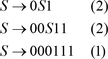
Consider the following context-free grammar:

which was designed to be able to generate the language L . L(G) is the notation for the language generated by the given grammar G :
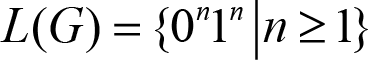
For example, obtaining 000111 can be done by starting with the Start symbol and consecutively applying the rules (2), (2) and (1) resulting in the following derivation :
A derivation in CFGs, which have rules in their rulesets involving more than one non-terminal (for example, ({ S },{+,1},{ S → S + S | S | 1}, S ) is called a left-most (right-most) derivation. At each step, we replace the left-most (right-most) non terminal:

thus obtaining the expression 1+1 and the parse tree (shown in Figure 4), which is an ordered tree representing the structure of the string according to the context-free grammar used to derive it.

|
| Figure 4 |
Push-down automaton
A push-down automaton can be imagined like a finite state-machine but with an extra stack attached to it. The following 7-tuple gives a more or less formal definition for it:

where:
- Q , Σ and F are defined likely as for a finite-state automaton
- Γ is the alphabet of the stack
- q 0 is the start state of the automaton
- Z 0 is the start symbol, Z 0 ∈ Γ
and the transition function is:

so it takes in a triplet of a state from Q , an input symbol (which can also be the empty string, called ϵ – epsilon) from Σ and a stack symbol from Γ and it gives a set of zero or more actions of the form ( p , α) where p is a state and α is a string of concatenated stack symbols.
Remembering the context-free grammar from our previous paragraph, we can construct a push-down automaton which will recognize the elements of {0 n 1 n | n ≥ 1}:

Concerning the states:
- q is the initial state and the automaton is in this state if it has not detected the symbol 1 so far but only 0s.
- p is the state where the automaton lies if it has detected at least one 1 and it can proceed forward only if there are 1s in the input.
- f is the final state
And where the transition function is defined as:
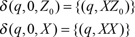
These two rules are handling the 0 from the input: both of them push one X onto the stack of the automaton for each 0 identified.
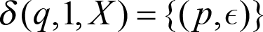
This rule will change to state p and pop one X from the stack
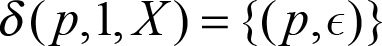
If in state p and we encounter a 1 in the input, pop one X from the stack
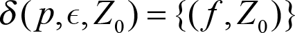
And finally, at this stage we have supposedly successfully identified our string of 0s and 1s. Our stack needs to be empty, the input fully consumed and then we can advance to the final state.
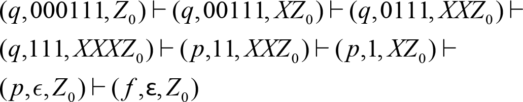
So, if we have 000111, the automaton goes through the following steps in order to recognize it as a valid input for the given grammar:
Now we can hopefully see the methodology involved in this step, we just need to create a push down automaton for our language which will successfully consume the series of tokens from the previous step thus resulting in a syntactically correct application.
In the paragraphs below, we frequently mention elements of a push-down automaton and refer to (context-free) grammars, hence this very short theoretical introduction. Unfortunately, a deeper study of this very exciting subject is beyond the scope of this article, being such a huge subject in the field of computer science that there are semester-long courses dedicated to the research of this domain. It is practically impossible for us to dig deeper into this field now. For everyone interested in this fascinating domain, I highly recommend Introduction to Automata Theory, Languages, and Computation by Hopcroft, Motwani and Ullman (2nd, 2001 edition).
The parser
The component responsible for this step in the compiler’s architecture is called the parser. Depending on the approach chosen to build the parse tree upon encountering an expression, we differentiate between the following types of parsers:
- descending – the tree is built from the root towards the leaves. In this situation, the parsing starts by applying consecutive transformations to the start symbol till we obtain the required expression. This approach is also called top-down parsing.
- ascending – the tree is built from the leaves towards the root, upon applying reverse transformations to the expression in order to reach the start symbol. This is also called bottom-up parsing.
Recursive-descent parsing
Usually the top-down parsers, which process the input from left to right, and the parse tree, which is constructed from top to bottom, are also known as recursive-descent parsers due to the recursive nature of context-free grammars. In the construction of the tree, a backtracking mechanism might be involved, which results in a less effective performance due to the constant back-stepping of the algorithm. These parsers are usually avoided in case of large grammars.
The parsers which are able to ‘predict’ which production is to be used on the input string do not require any backtracking steps and are called predictive parsers. These parsers operate on specialized LL ( k ) grammars, which are a simplified subset of the context-free grammars. Due to some applied restrictions and a precomputed state transition table introduced in the algorithm (which determines how to compute the next state from the current state and the lookahead symbol), they gain an extra simplicity when it comes to implementation.
LL ( k ) can be interpreted in the following manner:
- the first L means: L eft to right
- the second L means: L eft-most derivation
- and the k represents the number of lookaheads the parser can perform.
Parsers which operate on LL ( k ) grammars are also called LL ( k ) parsers.
Shift-reduce parsing
While reading the input, usually from left to right and trying to build up sequences on the stack which are recognized as the right side of a production, the parser can use two steps:
-
Reduce: Let’s consider the rule
A→w. When the stack containsqw, its content can be reduced toqA, whereAis a non-terminal from our grammar. When the entire content of the stack is reduced to the start symbol, we have successfully parsed the expression. - Shift: If we can’t perform a reduction (or ‘if we can’t reduce the stack’) of the stack, this step advances the input stream by one symbol, which is pushed onto the stack. This shifted symbol will be treated as a node in the parse tree.
Parsers using these steps are called shift-reduce parsers.
LR-parsers
A more performant family of the shift-reduce parsers are the LR parsers (invented by Donald Knuth in 1965 [ Knuth65 ]). They operate in linear time, producing correct results without backtracking on the input, using a L eft to right order and always use the R ight-most derivation in reverse. They are also known as LR ( k ) parsers, where k denotes the number of lookahead symbols the parser uses (which is mostly 1) in the decision-making step. Similarly to LL parsers, LR parsers use a state transition table that must be precomputed from the given grammar.
Several variants of the LR parsers are known:
- SLR parsers: these are the S imple LR parsers, categorized by a very small state transition table, working on the smallest grammars. They are easy to construct.
- LR (1)parser: these parsers work on large grammars. They have large generated tables, and they are theoretically enough to handle any reasonably constructed language – they are just slow to generate due to the huge state transition table.
- LALR (1) parsers: the L ook A head LR parsers are a simplified version of the LR parsers, able to handle intermediate size grammars, with the number of states being similar to SLR parsers.
LR parsers operate on LR grammars, whose pure theoretical definition we will skip for now. We will just mention that as per the [ Dragon ] book, page 242, the requirement of an LR ( k ) grammar states that “ we must be able to recognize the occurrence of the right side of a production in a right-sentential form with k input symbols of lookahead ” is less strict than the one for LL ( k ) grammars “ where we must be able to recognize the use of a production seeing only the first k symbols of what its right side derives ”. This allows LR grammars to describe a wider family of languages than LL grammars with only one drawback: the allowed complexity of the grammar makes it difficult to hand-construct a proper parser for it, so for a context-free grammar with a decent complexity, a parser generator will be required to generate a parser.
With this, we have ended our long but still frivolous journey in the world of parsers and syntax analysis, but for anyone interested there is no better source to turn to, than Chapter 4 of the dragon book [ Dragon ] where all these concepts are discussed in great length.
Semantic analysis
The semantic analysis stage during compilation validates the output generated by the syntax analysis and applies semantic rules to it in order to confirm the requirements of the language, such as strict type checking or other language-specific rules.
The input to this stage is an intermediate representation, mostly in the form of an abstract syntax tree created by the previous step, and the following operations may be performed on it, resulting in an annotated abstract syntax tree (or, if our product is a source-to-source translator, even the final variant of the result). The following list contains a few of the rules that can be applied in this stage; however, since semantic analysis is a highly programming-language-specific step, it is worth mentioning that each of the items can be prepended with ‘if the language has support for it then’:
- Type checking for various entities (such as, does the language require that indexes to an array must be a positive integer – for example, Pascal allows also negative indexes in the syntax).
- Validation of operands of various operators (some programming languages may consider having a multiplication sign between a string and an integer to be ill-formed to have, but not Python).
- Verification of implicit conversions (what will be the result of an addition of a real type variable to an integer type variable).
Code generation
In the last step of the compilation process, a typical compiler will generate executable code for the application. This is done by converting the resulting intermediate representation into a set of instructions (usually target architecture assembly, if we are compiling through assembly, or direct binary code).
The code generation phase, depending on the compiler itself, might be through the introduction and use of intermediate code, or some compilers can generate code directly for the target architecture. The intermediate code is a sort of machine code, which without being architecture specific can still represent the operations of the real machine.
The intermediate code is very often represented in the form of a 3-address code. The 3-address code can be viewed as a set of instructions where each instruction has at most 3 operands, and they are usually a combination of an assignment operation and a binary operation. For example, the following expression:
can be represented by the following sequence of 3-address code instructions:
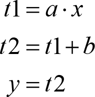
The importance of a 3-address code is that a very complex expression is broken down into several separate instructions which are very close to assembly level and they are very easily translated into the required machine code instruction.
Transforming an abstract syntax tree into a series of 3-address instructions is not an extremely complex task; basically, it just means traversing the tree and correctly identifying the set of temporaries and the values assigned to them, so generating code for the simple expressions of the language is possible using this process.
Generating code for compound statements, such as representing
IF
or
FOR
loops, usually boils down to a combination of jumps depending on the conditions imposed on the statements and then again generating code for simple expressions.
Generating code for function calls requires the presence of a stack, where – in the currently used Von Neumann architecture – we store not only the ingoing parameters to a function (if any) but also the addresses of return after the completion of the function.
First, the parameters are calculated, and their value is pushed onto the stack, then we issue the call command to invoke the method. This will also push the address where the called function should return after completing its execution. After the function has returned, we are back to the first instruction after the call of the method; the only thing that remains is to adjust the stack properly and continue execution.
Architecture of a compiler
For complex compiler projects, we usually see a three-stage structure like in Figure 5.

|
| Figure 5 |
This design has the advantage that several programming languages can be compiled using the same compiler (applying the same optimizations to all the source code written in different programming languages) to several machines and architectures (image courtesy of Wikipedia).
The front end
The front end section of the compiler is the one responsible for the lexical and syntax analysis of a dedicated programming language. It produces an intermediate representation of the program and should also manage the symbol table (which is a map of the symbols that were encountered in the program, such as variable names and function names, together with their location).
The lexical analysis, the syntax analysis and the semantic analysis steps are all part of the front end since these steps are all programming-language dependent.
If there is macro support in the language, the preprocessing phase is also part of the front end. The front end is responsible for creating an intermediate representation for further processing by the middle end.
The middle end
The middle end of the compiler is responsible for performing optimizations on the intermediary code. This is a platform and programming language independent operation, so all the programs compiled from languages that the compiler’s front end supports will benefit from this optimization phase. Some of the easiest to implement optimizations that can be performed on the intermediary code are in the section following, but for those interested in this subject [ CompOpt ] and [ Wikipedia-1 ] contain pretty exhaustive lists.
Constant folding and constant propagation
This optimization is responsible for finding values in code that occur in calculations that will never change during the lifetime of the application and for calculating them instead of doing the operations at runtime. for example:
  const int SECONDS_IN_HOUR = 60 * 60;
  const int SECONDS_IN_DAY = SECONDS_IN_HOUR * 24;
can be replaced with
const int SECONDS_IN_DAY = 86400;
where the value of
SECONDS_IN_HOUR
has been propagated to contain the correctly calculated (folding) value.
Dead code elimination
Sometimes there is a piece of code in the application which will not be reached. Dead code elimination will identify these cases and remove them, thus reducing the size of the code. For example:
  bool some_fun(int a)
  {
    if( a < 10)
    {
      return true;
    }
    else
    {
      return false;
    }
    std::cout << "some_fun exiting";
  }
In this case, the
std::cou
t will never be called, so the compiler is free to remove it.
Common sub-expression identification
This optimization is responsible for identifying calculations which are performed more than once. It extracts them into a commonly used part which can be inserted into the location where the calculation was done.
  int x = a + b + c;
  int z = a + b - d;
This can be optimized into the following sequence of code by extracting the common part
(a+b
) and reducing the generated code to the following:
  int temp = a + b;
  int x = temp + c;
  int z = temp - d;
These items are just a quick peek into the exhaustive list that an optimizing compiler does to your source code, so feel free to do more research in this field if you are interested in this fascinating domain.
The back end
The back end component of a compiler is the one which actually generates the code for the specified platform that this back end was written for. It receives the optimized intermediate representation (either an abstract syntax tree or a parse tree) from the middle end, and it may do some optimizations which are platform specific. In cases where is support for debugging the applications on the given platform, debug info is collected and inserted into the generated code.
As presented in the code generation paragraph, the abstract syntax tree is converted into a 3-address code representation, which the back end then re-works and re-organizes in order to represent the real computer architecture related concepts, such as registers, memory addresses, etc…
Modern compilers also have support for generating code for a specific platform (for example x86/64) but for different processor architecture, with the risk that the generated code will not run on anything else, but that specific processor, or it is possible to have the back end generate code for a totally different architecture (which process is called cross compilation).
Real-life compilers
In real life, it is a very frequent situation that a compiler is split up into several smaller applications, for example considering gcc , the following applications can be found on the system [ GCCArchitecture ]:
- gcc is a driver program which invokes the appropriate compilation application for the target language (for example cc1 being the preprocessor and the compiler for the C language, or gdc is the front end for the D language)
- as being the assembler (the assembler is the application which creates object (machine) code for specific compilation units), actually it is a part of the binutils package shipped with various systems
- collect2 is the linker (the application that creates a system specific binary from the various object files)
For clang , the overall system architecture and design is very similar to GCC , with the major difference being that clang was created with the aim of integration into various IDEs so there is a considerable set of libraries that make the project more flexible and easier to work with [ Guntli11 ], and also clang has the advantage of using the LLVM compiler infrastructure [ LLVM ].
For those not familiar with the terminology, LLVM used to stand for ‘Low Level Virtual Machine’, but right now it is just … LLVM, since the project outgrew the notion of a virtual machine, and evolved into a collection of various compiler-related artifacts that include a set of high quality components. This includes an implementation of the C++Standard Library to a debugger ( lldb ), and a set of front and back ends for various languages and target architectures via a powerful intermediate representation of the compiled language with a unique language (which is similar to assembly, and can be read by humans too) that the middle layer uses to perform strong optimizations on it before emitting architecture-specific code.
A script called primal
Now that we are done with the theoretical introduction of what a compiler is, how it works, and the algorithms and data structures behind the wall, it is time to sail into more practical waters, by introducing a small scripting language for which we create a compiler from scratch, and also a virtual machine to actually run the compiled code.
I mentioned that we will create the compiler from scratch although there is a plethora of tools available for this purpose. However, in my experience they have a tendency to generate code which is overly complex, difficult to read, and not suitable for our situation, where we want to explain the methodology of creating a compiler. Regardless, feel free to browse [ Wikipedia-4 ] to find a list of these tools stacked up against each other and find your favourite in there, dare you endeavour to create a new programming language.
The basic syntax
The script’s syntax is highly inspired by BASIC and for now it will support the following (very limited set of) operations:
- Mathematical operations: + (addition), - (subtraction), * (multiplication), / (division)
- Binary operations: & (and), | (or), ! (not), ^ (xor)
- Comparison operators: > (greater than), < (less than), == (equals), ≤ (less than or equals), ≥ (greater than or equals)
- Assignment operator: = (assignment)
And the following keywords will be implemented:
-
ifandthento verify the truthness of an expression (sadly, noelseis implemented yet) -
gototo hijack the execution flow by jumping to a specified label -
letto define a variable (if not found) and assign a value to it -
asmto directly tell the compiler to compile assembly syntax as per the VM’s opcodes (presented below) -
varto introduce a variable to the systemAs a side note, all variables need to be declared before they are used, à la Pascal. And for the moment, only numeric variables are supported.
-
endto close the code blocks of commands which have blocks (such asif) -
importto include the content of another source file into the current one
In order to define a label we use the following syntax:
:label
And as an extra feature, we will implement a
write
function which simply writes out what is passed in as parameters.
And now, armed with this knowledge we can write the following short application to print out a few Fibonacci numbers (see Listing 1).
import write

var t1, t2, nextTerm, n

let n = 100
let t1 = 0
let t2 = 1

:again

let nextTerm = t1 + t2

let t1 = t2
let t2 = nextTerm
if nextTerm < n then
    write(nextTerm, "  ")
    goto again
end
|
| Listing 1 |
As you have correctly observed, each line contains exactly one instruction. And also as you have observed, each line starts with a keyword. Both of these play an important role in the design of an application and will be explained later in the article.
In case you wish to compile scripts upon compilation, there are two executables in the build directory: primc is the compiler for the script language and primv is the virtual machine which runs the output of the compiler.
The Backus-Naur form of the primitive script
The Backus-Naur form is a notation scheme for context-free grammars, and it can be used to describe programming languages. Our own primitive script can be described (with a more complete version) of the following sequence of BNF (where
|
is used to indicate that only one can be chosen from the given set between
{
and
}
, the items between
[
and
]
are optional,
...
means a repetition of the previous group and
CR
means a newline).
I have omitted a few of the supported keywords from Listing 2 in order to not have the listing very long and boring; however, the example gives an overview of the complexity of how to start implementing the grammar required for a programming language, which in turn can be fed into a compiler compiler (for example yacc or bison) in order to generate a parser for the language.
<identifier>              ::= <letter>[{<letter>|<digit>}...]
<label identifier>        ::= <identifier>
<letter>                  ::= <small letter> | <capital letter>
<small letter>            ::= a|b|c|d|e|f|g|h|i|j|k|l|m|n|o|p|q|r|s|t|u|v|w|x|y|z
<capital letter>          ::= A|B|C|D|E|F|G|H|I|J|K|L|M|N|O|P|Q|R|S|T|U|V|W|X|Y|Z
<digit>                   ::= 0|1|2|3|4|5|6|7|8|9
<digit string>            ::= digit [{digit}...]
<label>                   ::= :<label identifier>
<immediate statement>     ::= <compound statement> CR
<compound statement>      ::= <statement> | <immediate statement>
<statement>               ::= let <identifier>=<expression>                   |
                              if <expression> then <compound statement> endif |
                              goto <label>                                    |
                              <label>                                         |
<comp op>                 ::= < | > | <= | >= | == | !=
<add op>                  ::= + | -
<mul op>                  ::= * | /
<expression>              ::= <term1> | <expression> \| <term1>
<term1>                   ::= <term2> | <term1> & <term2> | !<term2>
<term2>                   ::= <term3> | <term2> <comp op> <term3>
<term3>                   ::= <term4> | <term3> <add op> <term4>
<term4>                   ::= <term5> | <term4> <mul op> <term5>
<term5>                   ::= <term5> | <term5> ^ <term6>
<term6>                   ::= <expression> | <identifier> | <digit string>
|
| Listing 2 |
Our compiler
The project is a simple one-pass compiler, without any implemented optimizations. It was written in C++ and uses CMake as the build system. After you have checked out the project from https://github.com/fritzone/primal , you will find a directory structure, where the names of the directories are hopefully self-explanatory:
- compiler is where the compiler files are to be found
- vm stands for the source code for the virtual machine
- hal stands for the ‘Hardware Abstraction Layer’, just a fancy name
- opcodes stands for the assembly opcodes supported by the virtual machine
- tests is the directory of the unit tests, right now we use Catch2
But before we dig deeper here, just a quick mention: this entire project was created as a homegrown fun project, mostly for research purposes, so don’t expect production-quality speed (or code) neither from the compiler, nor from the compiled part. There are several excellent compilers in the market right now. I have tried to keep the primal compiler as simple and understandable as possible, and sometimes I had to cut a few corners to have it in a digestible size. For now, the entire project is released under an Affero GPL license, so feel free to modify, contribute and distribute in the spirit of true open source.
Banalities of the compiler
I had to create a few wrappers around common notions, such as ‘source’ in order to have an easier approach to them, but the entire project is packed in the primal namespace to not pollute the global one. As mentioned above, the compiler does not follow the standard mechanisms of creating a compiler, as we have not created a context-free grammar for it that can be fed into one of the automated tools to generate the proper mechanisms to automatically deal with situations that you can (will) encounter while writing a compiler. Instead, we tried to ‘guess’ how to approach these situations and ‘solved’ what had to be solved in a more manual manner, and – with explanations – they are presented here.
-
The compiler itself is located in the class
compiler. -
The source code is wrapped into the class
source. Very conveniently for us, this class usesstd::stringstreamto read in the required source code, from a string variable. As mentioned before, each line in the script lives its own life, and we have abused the string stream to serve us the text line by line by usingstd::getline. The text of the source is traversed only once. -
Each line of code is wrapped into a
class sequencederived keyword object. As mentioned before, in this programming language each line starts with a keyword, and these keywords are stored in their separate classes too, in the keywords folder inside the compiler. This decision was mainly influenced by the following- To keep it simple and easy to implement.
- To make it extensible without too much hassle – for example, introducing a new keyword should not be an extremely complex operation.
Parsing and tokenizing
For our little compiler, we have created a very simple tokenizer with a few lines of code, which suits very well our primitive script’s syntax. It can be found spread across the classes
lexer
,
parser
and
token
.
The
parser
class is responsible for parsing the entire source object that it was assigned, and the method
parser::parse
does the actual work:
  template<class CH> parse(source& input,
  CH checker, std::string& last_read) { ... }
The
checker
parameter has a specific role: the caller of the parse method can specify the condition at which the current sequence can stop. For the main compiler, this method is called like (from inside
compiler::compile
):
  std::string last;
  auto seqs = p.parse(m_src, [&](std::string) {
    return false;}, last);
however the implementation of the
if
keyword does something else:
  parser p;
  std::string last;
  auto seqs = p.parse(m_src,[&](std::string s)
    {
      return util::to_upper(s) == "END";
    },
    last);
  m_if_body = std::get<0>(seqs);
The reasoning is the following: in the primal language’s implementation, each keyword manages its own parsing and compilation, with some backup from the underlying architecture. So, the
if
keyword was responsible for extracting its own body (
m_if_body
) from the
source
object (
m_src
) and due to the syntax of the language, the body of the
if
is between the current position in the
m_src
and the corresponding
endif
keyword.
The inner workings of the
parser::parse
method are as follows:
std::string next_seq = input.next();
which will extract the next sequence of code (for us: next line) from the input (remember, this was of type
source
), and at the same time advance the location in the input. We see the result of the checker on the current sequence: if it evaluates to true, we will not continue the parsing but will go back to the entity which requested the parsing of the source from its specific location.
If we are still in the parsing phase, the tokenizer jumps in:
  lexer l(next_seq);
  std::vector<token> tokens = l.tokenize();
where the tokenize method is just a very rudimentary implementation of splitting a string into several components separated by space, comma or other characters. The result of the method is a vector of tokens, where each token has its own type that you can check out in token.h :
  enum class type
  {
    TT_OPERATOR  = 1, // omitting the rest
                      // to save space
The very first token, as per the definition of the language, must be a keyword. After tokenizing the sequence, we try to identify the keyword object and pass the control to it in order to prepare the sequence in the requested manner (for example, the way it was done for the
if
keyword is presented a few lines above). Different keywords do different preparations and checks, in order to validate the sequence.
When the keyword has successfully prepared and validated the sequence of tokens, it is time for us to run Edsger Dijkstra’s shunt-yard algorithm [ Dijkstra61 ] on it in order to obtain a reverse Polish notation from which we will construct the abstract syntax tree of the expression.
Building the ast is done in a recursive manner in
  static void build_ast(std::vector<token>& output,
  std::shared_ptr<ast>& croot);
where the parameter output is the actual output of the shuntyard algorithm:
  // create the RPN for the expression
  std::vector<token> output = shuntyard(tokens);
  // build the abstract syntax tree for the result
  // of the shuntyard
  ast::build_ast(output, seq->root());
Compiling
When the parsing is done, we get back the list of sequences – and by continuing our journey in
compiler::compile
we have reached the stage where we need to actually compile the sequences into the corresponding machine code. This is achieved by:
  // now compile the sequences coming from the parser
  for(const auto& seq : std::get<0>(seqs))
  {
    seq->compile(this);
  }
don’t let
std::get<0>(seqs)
scare you: as you can see in the source code,
parser::parse
actually returns a tuple of vector of sequences, where the first one means the instructions from the global namespace. Also, now you might want to jump down to the virtual machine section and read a bit about the architecture of it, to understand the instructions below, and come back after that.
As mentioned before, each keyword is required to compile its own code. Let’s present (in Listing 3), as an example, how the
if
keyword is actually doing its work (
kw_if::compile
).
// to compile the expression on which the IF takes
// its decision
sequence::compile(c);

// and set up the jumps depending on the trueness
// of the expression
label lbl_after_if =
  label::create(c->get_source());
label lbl_if_body =
  label::create(c->get_source());

// the comparator which evaluates the expression
comp* comparator =
  dynamic_cast<comp*>
  (operators[m_root->data.data()].get());

// generate code for the true case of it
(*c->generator()) << comparator->jump
  << lbl_if_body;
(*c->generator()) << DJMP() << lbl_after_if;

(*c->generator()) << declare_label(lbl_if_body);
for(const auto>amp; seq : m_if_body)
{
  seq->compile(c);
}
(*c->generator()) << declare_label(lbl_after_if);
|
| Listing 3 |
In the very first step: we compile this sequence via
sequence::compile(c);
to obtain the expression, the trueness of which is used by the if to decide whether to execute its body or not. Then we create two labels, one for the body of the
if
, the other one for the immediate location after the
if
.
Now, we obtain the comparator object from the root of the abstract syntax tree of this
if
object. At the current stage of the script (when writing this article), that must be a check for equality or comparison as no other operation is supported. The comparators are stored in the global map of
primal::operators
found in
operators.h
. This just lists all the operators the scripting language supports at the moment, together with the assembly opcode (more about this at a later stage, when we discuss the virtual machine) and a jump operation depending on the trueness of the operation.
The expression
*c->generator()
will yield a
generate
object which is actually a convenience class for seamlessly accessing (read: appending to) the
compiled_code
class, which is the part of the compiler where the compiled code actually resides.
Now that we have a
generate
object, first we output into it the
JUMP
operation (which is currently a jump depending on the state of a flag in the machine where this will run, which will be set depending on the trueness of the expression of the
if
) and the label of the body of the
if
.
After that, we output a direct jump to the first instruction after the body of the if (just in case the if was actually false).
Now it is time to compile the body of the
if
, and we are done.
Implementing the jumps
There is just one issue with compiling the jumps. Some of the labels might refer to locations/labels that at the current moment are not known because they come way after the current location. How this is solved currently is that the compiler inserts a bogus value at the location of the jump label, and in an internal map marks the spot of the label and its reference point. This happens in
generate::operator<<(const label& l)
.
When a label declaration happens, the compiler will finally know the location of the label, so it can update its map with the location in
generate::operator<<(declare_label &&dl)
.
When the compilation is done and all the locations of the labels are known,
compiled_code::finalize()
will patch the locations of the labels with the correct value.
The sequence compiler
At the very lowest level of the compiler is the sequence compiler found in
sequence::traverse_ast(uint8_t level, const std::shared_ptr<ast>& croot, compiler* c)
. This is responsible for compiling basic arithmetic expressions, dealing with numbers and variables, etc… The result – the compiled code – is actually a 3-address representation of the code, and the virtual machine interpreting the compiled bytecode was written to execute this representation.
This level tracks the variable index of the 3-address code. Initially, this starts at 0, is very conveniently mapped to registers in the virtual machine, and each descent in the abstract syntax tree will increment this. At the end of the traversal of the tree, the Reg(0) of the virtual machine will contain the value of the expression.
Depending on the type of the expression found in the current node of the tree, a different set of instructions is created. For example, the arithmetic operations generate the sequence of code shown in Listing 4.
if (croot->data.get_type() ==
  token::type::TT_OPERATOR)
{
  traverse_ast(level + 1, croot->left, c);
  (*c->generator()) << MOV() << reg(level)
    << reg(level + 1);
  traverse_ast(level + 1, croot->right, c);
  (*c->generator())
    << operators.at(croot->data.data())->opcode
    << reg(level) << reg(level + 1) ;
}
|
| Listing 4 |
To understand this piece of code, let’s consider that we are trying to compile the expression
2+3
.
This has yielded the following tokens, where
TT
stands for
T
oken
T
ype:
(2, TT_NUMBER)
,
(+, TT_OPERATOR)
and
(3, TT_NUMBER)
.
After shuntyarding the expression, we have the following reverse Polish notation:
(+, TT_OPERATOR)
,
(3, TT_NUMBER)
,
(2, TT_NUMBER)
.
This was transformed into the abstract syntax tree in Figure 6.

|
| Figure 6 |
Now we enter the
sequence::traverse_ast
method with the current root pointing to the root of the above tree, on level 0. The code sees that we actually have to deal with an operator:
+
.
It enters the
if
above, and it will immediately start descending into the tree on the next level, towards the left side of the tree. Now the current node points towards the
2
. The code sees that the data is actually a number, so it enters here:
  if (tt == token::type::TT_NUMBER)
  {
    (*c->generator()) << MOV() << reg(level)
      << croot->data;
  }
Now the following piece of code will be generated (which has the significance of initializing the register number 1 to 2):
MOV $r1 2
Since there is nothing more to be done here, we go back to the previous step (we were inside the
TT_OPERATOR if
branch), where the following instruction waits for us:
  (*c->generator()) << MOV() << reg(level)
    << reg(level + 1);
which will generate:
MOV $r0 $r1
ie. move the content of register 1 into register 0. Don’t forget that register 1 was initialized to 2 a few lines above. Now, we descend the tree to the right branch, where we see the
3
thus giving us the following:
MOV $r1 3
and we are done with that part too. Back to the inside of the
if
for
TT_OPERATOR
where the next operation is:
  (*c->generator())
    << operators.at(croot->data.data())->opcode
    << reg(level) << reg(level + 1)
This will go searching in the global
operators
table for the operator which is at the current level in the tree, and it will find the following row:
  ("+",  util::make_unique<ops> ("+", PRIO_10,
    new opcodes::ADD))
where the
opcodes::ADD
is the opcode responsible for executing addition in the system. So it will generate the following assembly code sequence:
ADD $r0 $r1
Since we are done with the tree, we are also done with the compilation, and we just exit. And at a very high level, this is the logic based on which the compiler is built.
There is just one drawback for this entire mechanism: since the virtual machine was built to have 256 registers (see below) at some point in very complex expressions, we simply might run out of registers. A resolution for future versions would be to implement the inclusion of a temporary variable in the code generation where the partial results are accumulated, but I reserve this for future enhancements of the compiler.
The assembly compiler
The script provides the programmer with the possibility of writing virtual-machine-specific assembly instructions. The keyword responsible for this is
asm
and the implementation is found in
kw_asm.cpp
. The build system generates a set of compiler files for the registered opcodes (please see below on how to register new opcodes) and a special component called the
asm_compiler
found in
asm_compiler.h
will generate the required code for the assembly instruction.
How to deal with the write function calls
As mentioned above, the function
write
is added to the system (see its source code in the
Appendix
) as a way to output data onto the screen. The
write
function is a dynamic function, meaning it can take in a various number and type of arguments (strings, variables and numbers) so I had to come up with a way to make it flexible enough to be usable.
One way to deal with it would have been the C way with a format string where various format specifiers are representing various interpretations of the data, but personally I’m not a great fan of it. Another way of dealing with this situation is presented by the Pascal compiler: while printing out, each type printed out is represented by a different function being called, and the compiler generates a list of method calls for all the parameters. Simple and effective. But unfortunately, at this moment I don’t have the infrastructure to support this.
So, I went in a third direction with this. With the help of the stack, I specify the number of parameters the function is having, then their type (string constant/number for now) and then the actual parameters. Now all is needed is just a clever write function which interprets the data from the stack, and all is done.
References
[CompOpt] Compiler optimizations: http://compileroptimizations.com/
[Dijkstra61] EdsgerW.Dijkstra (1961) ALGOL Bulletin Supplement no. 10 : http://www.cs.utexas.edu/~EWD/MCReps/MR35.PDF
[Dragon] Alfred V. Aho, Monica S. Lam, Ravi Sethi and Jeffrey D. Ullman (2006) Compilers: Principles, Techniques, and Tools
[GCCArchitecture] GNU C Compiler Architecture: https://en.wikibooks.org/wiki/GNU_C_Compiler_Internals/GNU_C_Compiler_Architecture
[Guntli11] Christopher Guntli (2011) ‘Architecture of clang’, https://wiki.ifs.hsr.ch/SemProgAnTr/files/Clang_Architecture_-_ChristopherGuntli.pdf
[Knuth65] Donald E. Knuth (July 1965). ‘On the translation of languages from left to right’. Information and Control 8(6): 607 - 639. doi: 10.1016/S0019 - 9958(65)90426-2
[LLVM] The LLVM Compiler Infrastructure: https://llvm.org/
[Wikipedia-1] Compiler optimizations: https://en.wikipedia.org/wiki/Category:Compiler_optimizations
[Wikipedia-2] Lexical analysis: https://en.wikipedia.org/wiki/Lexical_analysis
[Wikipedia-3] Multi-pass compiler: https://en.wikipedia.org/wiki/Multi-pass_compiler
[Wikipedia-4] Parser generators: https://en.wikipedia.org/wiki/Comparisonofparser_generators
[Wikipedia-5] Regular expression: https://en.wikipedia.org/wiki/Regular_expression
- Original diagram by Kenstruys (own work) and placed in the public domain. Gratefully downloaded from Wikimedia Commons https://commons.wikimedia.org/w/index.php?curid=6020058